import pandas as pd
import numpy as np
import matplotlib.pyplot as plt
import sklearn.tree
import sklearn.ensemble  ## 여러 트리 모듈을 이용하는 클래스를 포함

import matplotlib.animation  ## 그래프를 애니메이션으로 볼 예정
import IPython  ## IPython을 불러와서 산출...?

#-#
import warnings
warnings.filterwarnings('ignore')Bagging | 의사결정나무
Bagging
ensemble의Bagging을 이용해보자!
해당 포스트는 전북대학교 통계학과 최규빈 교수님의 강의내용을 토대로 재구성되었음을 알립니다.
1. 라이브러리 imports
2. 기본 의사결정나무로 데이터 적합
- 기온에 따른 아이스크림 판매량 데이터…
np.random.seed(43052)
temp = pd.read_csv('https://raw.githubusercontent.com/guebin/DV2022/master/posts/temp.csv').iloc[:,3].to_numpy()[:80]
temp.sort()
eps = np.random.randn(80)*3 # 오차
icecream_sales = 20 + temp * 2.5 + eps
df_train = pd.DataFrame({'temp':temp,'sales':icecream_sales})
df_train| temp | sales | |
|---|---|---|
| 0 | -4.1 | 10.900261 |
| 1 | -3.7 | 14.002524 |
| 2 | -3.0 | 15.928335 |
| 3 | -1.3 | 17.673681 |
| 4 | -0.5 | 19.463362 |
| ... | ... | ... |
| 75 | 9.7 | 50.813741 |
| 76 | 10.3 | 42.304739 |
| 77 | 10.6 | 45.662019 |
| 78 | 12.1 | 48.739157 |
| 79 | 12.4 | 46.007937 |
80 rows × 2 columns
## step 1
X = df_train[['temp']]
y = df_train['sales']

## step 2
tree = sklearn.tree.DecisionTreeRegressor()  ## 완전 퓨어하게, 하이퍼파라미터도 건드리지 말고.

## step 3
tree.fit(X, y)DecisionTreeRegressor()In a Jupyter environment, please rerun this cell to show the HTML representation or trust the notebook.
On GitHub, the HTML representation is unable to render, please try loading this page with nbviewer.org.
DecisionTreeRegressor()
plt.plot(X, y, 'o')
plt.plot(X, tree.predict(X), '--')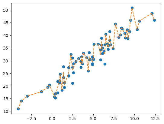
우리가 지금까지 먹어왔던 기본적인
DecisionTreeRegressor()이다. 오차항까지 그대로 따라가는 모습이 참으로 안타깝다…
3. 배깅
- 같은 자료를 배깅을 이용해 적합한다면…
## step 1
X = df_train[['temp']]
y = df_train['sales']

## step 2
predictr = sklearn.ensemble.BaggingRegressor()  ## 앙상블의 배깅 리그레서

## step 3
predictr.fit(X, y)BaggingRegressor()In a Jupyter environment, please rerun this cell to show the HTML representation or trust the notebook.
On GitHub, the HTML representation is unable to render, please try loading this page with nbviewer.org.
BaggingRegressor()
fig, ax = plt.subplots(1,2, figsize = (13,5))
ax[0].plot(X, y, 'o', label = 'True')
ax[0].plot(X, tree.predict(X), '--', label = 'prediction')
ax[0].set_title('Pure Tree')
ax[0].legend()

ax[1].plot(X, y, 'o', label = 'True')
ax[1].plot(X, predictr.predict(X), '--', label = 'prediction')
ax[1].set_title('Bagging')
ax[1].legend()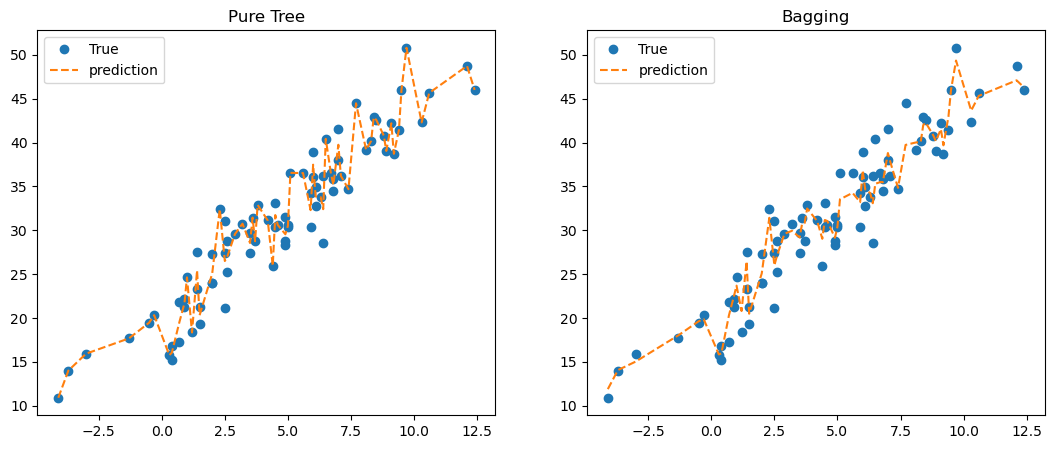
뭔가 무지성적인 오차항 추종이 옅어졌다…?!
4. 배깅의 원리에 대한 분석
기본원리
- 알고리즘
- n개의 샘플에서 n개를 무작위로 복원추출한다. 부트스트랩(Bootstrap)!!
- 1번에서 뽑힌 샘플들을 이용하여
tree를 적합한다. - 상기 과정을 10번 반복하고, 10개의
tree의 평균값을yhat으로 택한다.
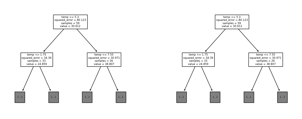
A. plot_tree 체크
- 10개의 트리들의 리스트를 찾으려면?
trees = predictr.estimators_
trees
[DecisionTreeRegressor(random_state=1644635363),
DecisionTreeRegressor(random_state=1304269235),
DecisionTreeRegressor(random_state=1794000214),
DecisionTreeRegressor(random_state=1273087880),
DecisionTreeRegressor(random_state=995922005),
DecisionTreeRegressor(random_state=1372517728),
DecisionTreeRegressor(random_state=1087222928),
DecisionTreeRegressor(random_state=3687756),
DecisionTreeRegressor(random_state=1772778467),
DecisionTreeRegressor(random_state=92158766)]정말 말그대로 표본마다 각각
DecisionTreeRegressor()로 적합해준 것이다.
- 재표본의 데이터셋을 찾으려면? (부트스트랩 샘플 인덱스)
predictr.estimators_samples_[array([19, 10, 25, 29, 50, 7, 46, 31, 10, 39, 78, 14, 54, 79, 28, 35, 73,
0, 74, 72, 66, 36, 55, 24, 41, 11, 68, 65, 71, 36, 54, 41, 76, 34,
0, 59, 5, 7, 67, 61, 64, 21, 27, 26, 43, 55, 49, 23, 29, 27, 41,
14, 58, 5, 12, 40, 12, 38, 8, 19, 63, 4, 35, 75, 64, 9, 69, 17,
32, 15, 60, 55, 18, 55, 22, 73, 28, 48, 57, 63]),
array([51, 70, 43, 33, 42, 76, 13, 32, 39, 6, 44, 32, 78, 38, 54, 4, 54,
78, 75, 1, 59, 58, 26, 41, 21, 45, 45, 63, 15, 0, 45, 43, 24, 50,
77, 26, 51, 53, 38, 6, 22, 5, 10, 32, 76, 7, 46, 70, 40, 28, 64,
69, 32, 49, 1, 1, 37, 7, 29, 29, 22, 1, 50, 56, 44, 52, 0, 30,
32, 73, 53, 69, 78, 46, 12, 3, 18, 60, 41, 70]),
array([55, 8, 0, 71, 14, 74, 10, 7, 58, 10, 0, 50, 23, 61, 36, 66, 66,
52, 17, 6, 36, 3, 55, 13, 41, 5, 77, 21, 31, 14, 19, 59, 3, 25,
79, 39, 18, 24, 55, 5, 57, 19, 40, 15, 3, 75, 36, 25, 22, 13, 53,
55, 71, 28, 7, 1, 68, 48, 49, 77, 34, 35, 66, 41, 72, 45, 23, 63,
34, 50, 68, 47, 28, 20, 37, 23, 67, 17, 71, 64]),
array([ 8, 24, 8, 32, 8, 37, 58, 59, 68, 32, 37, 16, 34, 55, 14, 2, 43,
39, 77, 16, 71, 24, 5, 71, 26, 43, 8, 12, 13, 10, 54, 3, 36, 23,
67, 3, 42, 48, 6, 34, 49, 30, 50, 33, 57, 54, 72, 56, 57, 62, 6,
36, 34, 75, 33, 66, 1, 39, 61, 61, 7, 49, 23, 35, 10, 67, 54, 74,
58, 23, 11, 42, 37, 1, 16, 79, 11, 6, 34, 44]),
array([51, 62, 23, 0, 1, 67, 70, 71, 56, 31, 4, 38, 22, 10, 6, 31, 66,
19, 67, 72, 75, 17, 3, 21, 16, 44, 59, 8, 58, 27, 25, 17, 14, 17,
27, 6, 36, 77, 37, 46, 30, 1, 34, 7, 78, 23, 68, 22, 49, 26, 14,
38, 48, 3, 63, 5, 4, 71, 74, 32, 41, 59, 22, 37, 57, 71, 56, 30,
15, 28, 52, 42, 50, 79, 14, 15, 44, 37, 50, 76]),
array([63, 61, 25, 22, 15, 19, 39, 5, 3, 48, 38, 68, 41, 48, 32, 45, 34,
52, 26, 2, 4, 7, 14, 59, 47, 79, 19, 48, 1, 66, 3, 4, 61, 65,
10, 1, 19, 55, 11, 60, 17, 71, 40, 0, 2, 27, 17, 67, 22, 74, 13,
71, 48, 37, 72, 58, 48, 44, 59, 32, 28, 53, 28, 39, 18, 0, 7, 6,
54, 0, 47, 47, 57, 66, 23, 66, 32, 77, 26, 34]),
array([16, 22, 69, 63, 3, 32, 20, 66, 53, 5, 27, 1, 51, 1, 47, 41, 41,
33, 14, 7, 54, 27, 57, 75, 64, 8, 7, 8, 26, 41, 24, 44, 70, 65,
66, 42, 54, 76, 50, 67, 15, 62, 19, 42, 38, 71, 53, 45, 23, 72, 65,
24, 69, 47, 0, 75, 29, 34, 23, 63, 33, 77, 69, 18, 65, 2, 79, 33,
37, 58, 26, 55, 58, 63, 45, 17, 77, 41, 54, 13]),
array([76, 31, 49, 79, 34, 63, 18, 30, 12, 35, 8, 46, 50, 49, 43, 13, 19,
68, 79, 4, 13, 22, 12, 76, 53, 52, 8, 31, 40, 39, 22, 53, 48, 15,
64, 19, 40, 1, 54, 77, 38, 28, 31, 71, 38, 42, 27, 6, 18, 42, 34,
0, 75, 37, 16, 58, 60, 62, 18, 2, 74, 6, 5, 65, 77, 44, 4, 9,
24, 15, 71, 59, 23, 37, 76, 68, 70, 65, 34, 73]),
array([70, 27, 42, 10, 74, 26, 0, 51, 2, 12, 23, 28, 38, 30, 6, 32, 63,
73, 23, 68, 8, 79, 43, 68, 15, 44, 34, 55, 33, 0, 51, 66, 66, 47,
53, 76, 27, 3, 71, 10, 70, 30, 79, 1, 25, 49, 18, 0, 17, 65, 14,
27, 29, 76, 15, 12, 31, 26, 61, 42, 41, 21, 22, 38, 31, 11, 23, 13,
25, 10, 41, 23, 78, 73, 77, 47, 42, 32, 34, 5]),
array([46, 24, 65, 62, 70, 15, 15, 33, 39, 44, 16, 33, 50, 24, 31, 36, 3,
69, 8, 34, 29, 72, 59, 30, 48, 63, 51, 45, 26, 74, 65, 48, 77, 26,
43, 55, 9, 28, 33, 35, 44, 25, 51, 6, 47, 56, 50, 72, 74, 47, 60,
8, 50, 9, 31, 10, 79, 45, 28, 61, 43, 55, 19, 73, 15, 19, 53, 46,
13, 70, 41, 57, 34, 62, 34, 59, 18, 30, 43, 16])]길이가 80인
array들의 리스트로 나타난다. 이것들은 데이터의 인덱스를 의미하는 것이므로 데이터프레임에loc을 해주면 뽑아낼 수 있다…
사실 엄밀히 말하자면 해당 데이터를 가지고 피팅을 하는 건 아니고, 인덱스의 수를 골라서 가중치를 부여하는 방식으로 들어가긴 한다…
- 첫번째 트리(predictr.estimators_[0]) 재현
## 호출하기 쉽도록 변수들을 어레이로 바꿔줌
X_arr = np.array(X)
y_arr = np.array(y)

## 적합
tree = sklearn.tree.DecisionTreeRegressor()
tree.fit(X_arr[predictr.estimators_samples_[0]], y_arr[predictr.estimators_samples_[0]])DecisionTreeRegressor()In a Jupyter environment, please rerun this cell to show the HTML representation or trust the notebook.
On GitHub, the HTML representation is unable to render, please try loading this page with nbviewer.org.
DecisionTreeRegressor()
sklearn.tree.plot_tree(
    tree,
    max_depth = 1,
    feature_names = X.columns.to_list()
);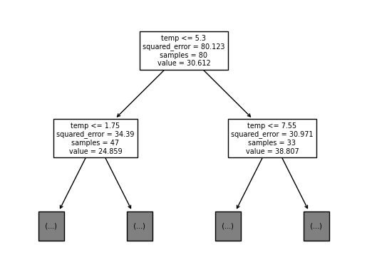
## 작업결과
sklearn.tree.plot_tree(
    predictr.estimators_[0],
    feature_names = X.columns.to_list(),
    max_depth = 1
);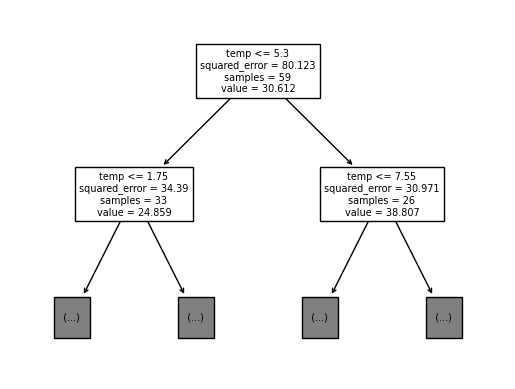
실제 작업된 결과와 동일한 것을 알 수 있다.
다만,
Bagging에서는.fit(sample_weight)를 지정하여 가중치로 데이터의 수를 설정하기 때문에samples의 사이즈는 다르다.
- 엄밀하게 해보면…
## 정확히는 sample_weight를 조정하는 것
## 이런 식으로...
lst = list(np.zeros(len(X)))

for i in predictr.estimators_samples_[0] :
    lst[i] = lst[i] + 1
tree.fit(X, y, sample_weight = lst)

fig, ax = plt.subplots(1,2, figsize = (13, 5))
sklearn.tree.plot_tree(
    predictr.estimators_[0],
    feature_names = X.columns.to_list(),
    max_depth = 1,
    ax = ax[0]
)
sklearn.tree.plot_tree(
    tree,
    feature_names = X.columns.to_list(),
    max_depth = 1,
    ax = ax[1]
);
이러니까 하나도 차이가 없지요잉?
- tree와 predictr의 트리플랏 비교 (고정된 i)
i = 4

fig, ax = plt.subplots(2,1)

sklearn.tree.plot_tree(
    predictr.estimators_[i],
    feature_names = X.columns.to_list(),
    max_depth = 1,
    ax = ax[0]
)
ax[0].set_title('Bagging Predictor')

tree = sklearn.tree.DecisionTreeRegressor()
tree.fit(X_arr[predictr.estimators_samples_[i]], y_arr[predictr.estimators_samples_[i]])  ## 가중치 없는 퓨어 트리모델
sklearn.tree.plot_tree(
    tree,
    feature_names = X.columns.to_list(),
    max_depth = 1,
    ax = ax[1]
)
ax[1].set_title('tree')
Text(0.5, 1.0, 'tree')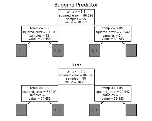
- tree와 predictr간 트리플랏 비교(애니메이션)
fig, ax = plt.subplots(2, 1)
plt.close()
def func(frame) :
ax[0].clear() ## 배깅으로 적합한 predictr
sklearn.tree.plot_tree(
predictr.estimators_[frame],
feature_names = X.columns.to_list(),
max_depth = 1,
ax = ax[0]
)
ax[0].set_title('Bagging Predictor')
ax[1].clear() ## 퓨어 의사결정나무로 적합한 predictr
tree = sklearn.tree.DecisionTreeRegressor()
tree.fit(X_arr[predictr.estimators_samples_[frame]], y_arr[predictr.estimators_samples_[frame]])
sklearn.tree.plot_tree(
tree,
feature_names = X.columns.to_list(),
max_depth = 1,
ax = ax[1]
)
ax[1].set_title('Pure Tree')ani = matplotlib.animation.FuncAnimation(
fig,
func,
frames = 10
)
display(IPython.display.HTML(ani.to_jshtml()))모든 프레임의 위 아래 값이 samples의 값만을 제외하고 동일한 모습이다. (샘플을 동일하게 만들고 싶다면 위에서 언급한 과정을 사용하라. 바꾸기 귀찮아서 생략하나, 충분히 수행할 수 있을 것이다…)
## B. Resampling + Fit
- estimator에 따라 달라지는 예측치
samples = predictr.estimators_samples_
trees = [sklearn.tree.DecisionTreeRegressor() for i in range(len(predictr.estimators_))]
for i in range(len(predictr.estimators_)) :
    trees[i].fit(X_arr[predictr.estimators_samples_[i]], y_arr[predictr.estimators_samples_[i]])

i = 0  ## i번째 estimator, 해당 값을 바꿔가며 그래프를 확인해보자.
plt.plot(X, y, 'o', alpha = 0.2, color = 'grey', label = 'True')  ## 실제값
plt.plot(X_arr[samples[i]], y_arr[samples[i]], 'o', alpha = 0.33, label = 'Resample')  ## 리샘플링된 값, true값과 겹침
plt.plot(X, trees[i].predict(X), '--', label = 'Prediction')  ## X에 대한 예측값
plt.legend()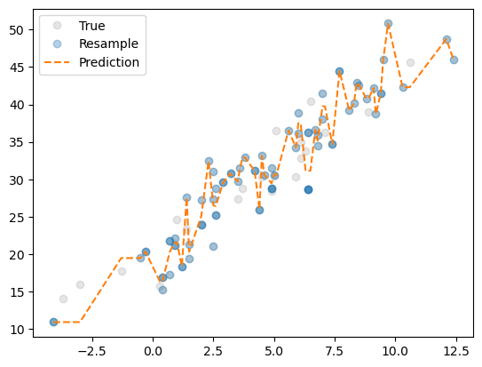
어떤 샘플이 뽑히냐에 따라 (
i의 값이 달라질 때마다) 적합되는 모양이 달라진다.
- 달라지는 양상을 애니메이션으로 시각화
fig, ax = plt.subplots(1)
plt.close()
def func(frame) :
ax.clear()
ax.plot(X, y, 'o', alpha = 0.2, color = 'grey', label = 'True')
ax.plot(X_arr[samples[frame]], y_arr[samples[frame]], 'o', alpha = 0.3, label = 'Resampled')
ax.plot(X, trees[frame].predict(X), '--', label = 'Prediction')
ax.legend()ani = matplotlib.animation.FuncAnimation(
fig,
func,
frames = 10
)
display(IPython.display.HTML(ani.to_jshtml())) ## IPython에서 HTML을 인코딩해옴.C. 앙상블결과 재현
- 손코딩으로 직접 풀어보자…
Bagging으로 예측한 값
predictr.predict(X)array([11.88782962, 14.05941305, 15.02231867, 18.03161729, 19.62619066,
19.86214551, 15.84293717, 15.95940294, 15.95940294, 20.30137042,
20.30137042, 22.51278676, 22.51278676, 23.68899036, 20.7954938 ,
26.45727462, 26.45727462, 20.48421278, 20.48421278, 25.08188452,
25.08188452, 25.08188452, 31.42611771, 25.99393577, 25.99393577,
25.99393577, 27.05912187, 27.05912187, 29.60439358, 29.94005816,
29.18760881, 29.18760881, 30.75340115, 30.82608162, 32.48384789,
31.03678302, 29.02978839, 31.17487146, 31.17487146, 31.05349512,
29.147739 , 29.147739 , 29.147739 , 30.40843883, 30.40843883,
33.53154643, 34.26668831, 33.20982041, 33.20982041, 36.82818648,
36.82818648, 34.66545508, 34.66545508, 34.24047203, 33.0829342 ,
33.0829342 , 35.29894866, 35.50366771, 35.47938512, 35.47938512,
38.8116606 , 38.8116606 , 37.74794717, 34.84063828, 39.73515434,
40.01130524, 40.05274675, 41.9980937 , 42.26869452, 40.81707653,
40.16985211, 41.5373848 , 39.69311797, 42.97563198, 45.99122302,
49.35681519, 43.64765096, 45.32629064, 47.10042494, 46.28105912])- 열 개의 트리로 예측한 값의 평균
np.stack([tree.predict(X) for tree in predictr.estimators_]).shape, np.array([tree.predict(X) for tree in predictr.estimators_]).mean(axis = 0).shape((10, 80), (80,))np.array([tree.predict(X) for tree in predictr.estimators_]).mean(axis = 0) ## 행마다 평균을 내어 하나의 어레이로 만듦array([11.88782962, 14.05941305, 15.02231867, 18.03161729, 19.62619066,
19.86214551, 15.84293717, 15.95940294, 15.95940294, 20.30137042,
20.30137042, 22.51278676, 22.51278676, 23.68899036, 20.7954938 ,
26.45727462, 26.45727462, 20.48421278, 20.48421278, 25.08188452,
25.08188452, 25.08188452, 31.42611771, 25.99393577, 25.99393577,
25.99393577, 27.05912187, 27.05912187, 29.60439358, 29.94005816,
29.18760881, 29.18760881, 30.75340115, 30.82608162, 32.48384789,
31.03678302, 29.02978839, 31.17487146, 31.17487146, 31.05349512,
29.147739 , 29.147739 , 29.147739 , 30.40843883, 30.40843883,
33.53154643, 34.26668831, 33.20982041, 33.20982041, 36.82818648,
36.82818648, 34.66545508, 34.66545508, 34.24047203, 33.0829342 ,
33.0829342 , 35.29894866, 35.50366771, 35.47938512, 35.47938512,
38.8116606 , 38.8116606 , 37.74794717, 34.84063828, 39.73515434,
40.01130524, 40.05274675, 41.9980937 , 42.26869452, 40.81707653,
40.16985211, 41.5373848 , 39.69311797, 42.97563198, 45.99122302,
49.35681519, 43.64765096, 45.32629064, 47.10042494, 46.28105912])위에서의 예측은 개별 트리의 예측값들의 평균으로 정리되었다는 것을 알 수 있다.
- 최종결과물 (코드로 정리)
def ensemble(trees, i=None) :
    if i is None :
        i = len(trees)  ## i가 Null일 때, trees의 length로 설정
    yhat = np.array([tree.predict(X) for tree in predictr.estimators_[:i+1]]).mean(axis = 0)  ## i+1까지 슬라이싱하는 거니까 i번째까지 뽑는다.
    return yhat
i의 의미… 몇 번째 트리까지만 결과값을 산출하는 데에 이용하겠음… 디폴트는 전부 다…(10개)
- 예시 : 0번 트리의 예측값 평균만 활용
ensemble(trees, 0) ## 0번 트리만 적용array([10.90026146, 10.90026146, 10.90026146, 19.46336233, 19.46336233,
20.31785349, 16.3076088 , 16.3076088 , 16.3076088 , 20.27763408,
20.27763408, 21.52796629, 21.52796629, 21.52796629, 18.34698175,
27.5369675 , 27.5369675 , 20.30881248, 20.30881248, 25.04963215,
25.04963215, 25.04963215, 32.42440294, 26.49340711, 26.49340711,
26.49340711, 26.40925726, 26.40925726, 29.55903213, 30.75418385,
29.70592592, 29.70592592, 31.45007539, 32.89828946, 32.89828946,
31.12503261, 25.9552363 , 33.12203011, 33.12203011, 30.60313283,
29.45886461, 29.45886461, 29.45886461, 30.60789344, 30.60789344,
30.60789344, 36.5245913 , 34.24458444, 34.24458444, 37.4829917 ,
37.4829917 , 37.4829917 , 37.4829917 , 31.13974993, 31.13974993,
31.13974993, 31.13974993, 36.58400962, 35.1723381 , 35.1723381 ,
39.75311187, 39.75311187, 39.75311187, 34.68877582, 44.47780794,
39.1744058 , 40.19626989, 42.86734269, 42.60143843, 40.80476673,
40.80476673, 42.1996627 , 38.72741866, 41.43992372, 45.95732063,
50.81374143, 42.30473921, 42.30473921, 48.7391566 , 46.00793717])- 9번 트리(마지막 트리)의 예측값까지 활용(전부 다)
display(str(ensemble(trees, 9)) == str(ensemble(trees)))
display(ensemble(trees, 9))Truearray([11.88782962, 14.05941305, 15.02231867, 18.03161729, 19.62619066,
19.86214551, 15.84293717, 15.95940294, 15.95940294, 20.30137042,
20.30137042, 22.51278676, 22.51278676, 23.68899036, 20.7954938 ,
26.45727462, 26.45727462, 20.48421278, 20.48421278, 25.08188452,
25.08188452, 25.08188452, 31.42611771, 25.99393577, 25.99393577,
25.99393577, 27.05912187, 27.05912187, 29.60439358, 29.94005816,
29.18760881, 29.18760881, 30.75340115, 30.82608162, 32.48384789,
31.03678302, 29.02978839, 31.17487146, 31.17487146, 31.05349512,
29.147739 , 29.147739 , 29.147739 , 30.40843883, 30.40843883,
33.53154643, 34.26668831, 33.20982041, 33.20982041, 36.82818648,
36.82818648, 34.66545508, 34.66545508, 34.24047203, 33.0829342 ,
33.0829342 , 35.29894866, 35.50366771, 35.47938512, 35.47938512,
38.8116606 , 38.8116606 , 37.74794717, 34.84063828, 39.73515434,
40.01130524, 40.05274675, 41.9980937 , 42.26869452, 40.81707653,
40.16985211, 41.5373848 , 39.69311797, 42.97563198, 45.99122302,
49.35681519, 43.64765096, 45.32629064, 47.10042494, 46.28105912])### D. 학습과정(steps) 시각화
- 고정된 i
i = 0

fig, ax = plt.subplots(1,4, figsize = (13, 3))
## step 0 -- data import
ax[0].set_title('Step 0')
ax[0].plot(X, y, 'o', color = 'grey', alpha = 0.2)

## step 1 -- Resampling
ax[1].set_title('Step 1 : ReSampling')
ax[1].plot(X, y, 'o', color = 'grey', alpha = 0.2)
ax[1].plot(X_arr[samples[i]], y_arr[samples[i]], 'o', alpha = 0.3)

## step 2 -- fitting
ax[2].set_title('Step 3 : Fitting')
ax[2].plot(X, y, 'o', color = 'grey', alpha = 0.2)
ax[2].plot(X_arr[samples[i]], y_arr[samples[i]], 'o', alpha = 0.3)
ax[2].plot(X, trees[i].predict(X), '--')  ## 개별 tree의 적합

## step 3 -- ensemble
ax[3].set_title('Step 4 : Ensemble')
ax[3].plot(X, y, 'o', color = 'grey', alpha = 0.2)
ax[3].plot(X, ensemble(trees, i), '--')  ## 적합한 트리들을 평균내어 적용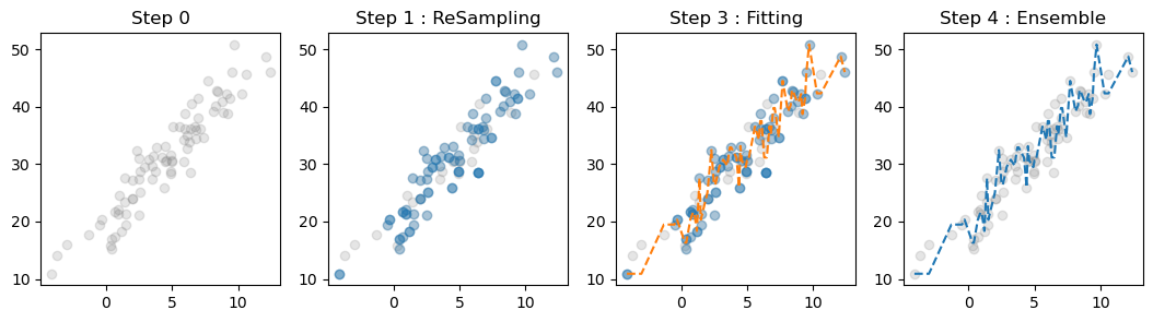
Bagging이 적합하는 과정 :
- 자료를 받아온다.
- 받아온 자료를 복원추출한다.
- 복원추출한 자료를 의사결정나무로 적합한다.
- 적합한 트리들의 개별 예측값들의 평균을 최종 예측값으로 제시한다.
- 애니메이션화
def func(i) :
    for a in ax:
        a.clear()

    ## step 0 -- data import
    ax[0].set_title('Step 0')
    ax[0].plot(X, y, 'o', color = 'grey', alpha = 0.2)

    ## step 1 -- Resampling
    ax[1].set_title('Step 1 : ReSampling')
    ax[1].plot(X, y, 'o', color = 'grey', alpha = 0.2)
    ax[1].plot(X_arr[samples[i]], y_arr[samples[i]], 'o', alpha = 0.3)

    ## step 2 -- fitting
    ax[2].set_title('Step 3 : Fitting')
    ax[2].plot(X, y, 'o', color = 'grey', alpha = 0.2)
    ax[2].plot(X_arr[samples[i]], y_arr[samples[i]], 'o', alpha = 0.3)
    ax[2].plot(X, trees[i].predict(X), '--')  ## 개별 tree의 적합

    ## step 3 -- ensemble
    ax[3].set_title('Step 4 : Ensemble')
    ax[3].plot(X, y, 'o', color = 'grey', alpha = 0.2)
    ax[3].plot(X, ensemble(trees, i), '--', color = 'C1')
ani = matplotlib.animation.FuncAnimation(
fig,
func,
frames = len(predictr.estimators_features_)
)
display(IPython.display.HTML(ani.to_jshtml()))최종 예측값에 관여하는
tree의 수가 많아질수록 예측값의 선이 완만해진다…
5. 어떻게 이런 생각을 했을까?
# 모티브 : 끝자락의 예측값들을 조금 완만하게 만들고 싶었고, 이를 서로 다른 여러개의 tree를 만들어 해결하고자 하는데, 붓스트랩에서 영감을 받아 여러개의 트리를 만들었다.
# 오차까지 적합하려고 하는 의사결정나무의 작동방식을 완화하려고 했음.